1
2
3
4
5
6
7
8
9
10
11
12
13
14
15
16
17
18
19
20
21
22
23
24
25
26
27
28
29
30
31
32
33
34
35
36
37
38
39
40
41
42
43
44
45
46
47
48
49
50
51
52
53
54
55
56
57
58
59
60
61
62
|
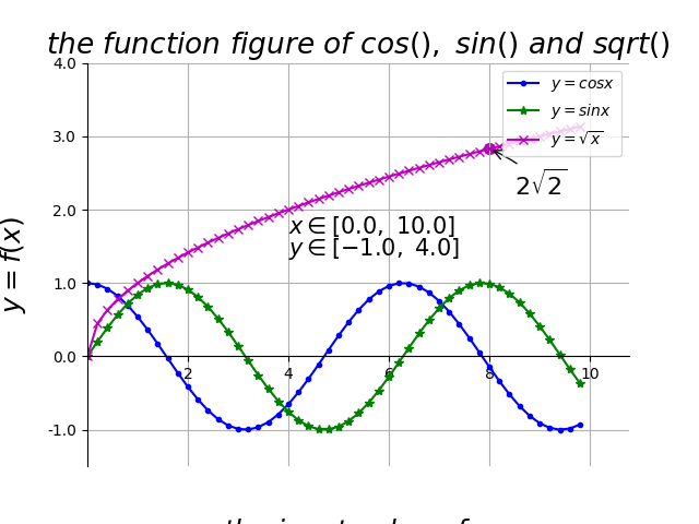
import numpy as np
import matplotlib.pyplot as plt
from pylab import *
x = np.arange(0., 10, 0.2)
y1 = np.cos(x)
y2 = np.sin(x)
y3 = np.sqrt(x)
plt.plot(x, y1, color='blue', linewidth=1.5, linestyle='-', marker='.', label=r'$y = cos{x}$')
plt.plot(x, y2, color='green', linewidth=1.5, linestyle='-', marker='*', label=r'$y = sin{x}$')
plt.plot(x, y3, color='m', linewidth=1.5, linestyle='-', marker='x', label=r'$y = \sqrt{x}$')
ax = plt.subplot(111)
ax.spines['right'].set_color('none')
ax.spines['top'].set_color('none')
ax.xaxis.set_ticks_position('bottom')
ax.spines['bottom'].set_position(('data', 0))
ax.yaxis.set_ticks_position('left')
ax.spines['left'].set_position(('data', 0))
plt.xlim(x.min()*1.1, x.max()*1.1)
plt.ylim(-1.5, 4.0)
plt.xticks([2, 4, 6, 8, 10], [r'2', r'4', r'6', r'8', r'10'])
plt.yticks([-1.0, 0.0, 1.0, 2.0, 3.0, 4.0],
[r'-1.0', r'0.0', r'1.0', r'2.0', r'3.0', r'4.0'])
plt.text(4, 1.68, r'$x \in [0.0, \ 10.0]$', color='k', fontsize=15)
plt.text(4, 1.38, r'$y \in [-1.0, \ 4.0]$', color='k', fontsize=15)
plt.scatter([8,],[np.sqrt(8),], 50, color ='m')
plt.annotate(r'$2\sqrt{2}$', xy=(8, np.sqrt(8)), xytext=(8.5, 2.2), fontsize=16, color='#090909', arrowprops=dict(arrowstyle='->', connectionstyle='arc3, rad=0.1', color='#090909'))
plt.title(r'$the \ function \ figure \ of \ cos(), \ sin() \ and \ sqrt()$', fontsize=19)
plt.xlabel(r'$the \ input \ value \ of \ x$', fontsize=18, labelpad=88.8)
plt.ylabel(r'$y = f(x)$', fontsize=18, labelpad=12.5)
plt.legend(loc='upper right')
plt.grid(True)
plt.savefig("../img/2019-06-24_Matplotlib基本语法_1.png")
plt.close()
|