线性回归
创建数据
1 | def make_data(nDim): |
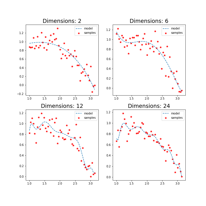
最小二乘法 Ordinary Least Squares (OLS)
目标函数:
不足:OLS为了更好的拟合数据,会使用较大的w值,进而导致过度拟合。
1 | import matplotlib.pyplot as plt |
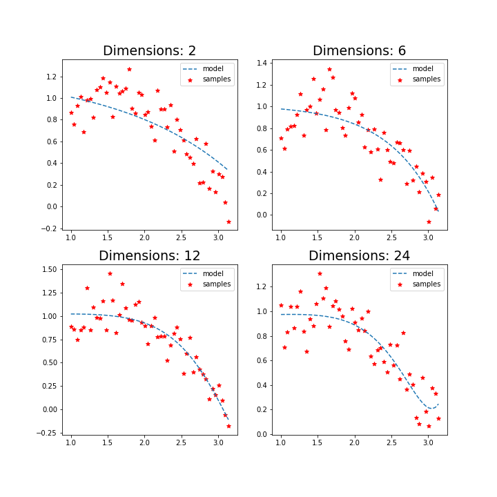
岭回归 Ridge Regression (Tikhonov Regularization)
目标函数:
优化:为惩罚OLS每个w逐渐增加导致过度拟合的问题,新增的项为L2惩罚项(L2 Penalty)。
特点:w有可能特别小的绝对值,但很难达成0,造成贡献很小的系数还是要放,影响性能。
1 | import matplotlib.pyplot as plt |
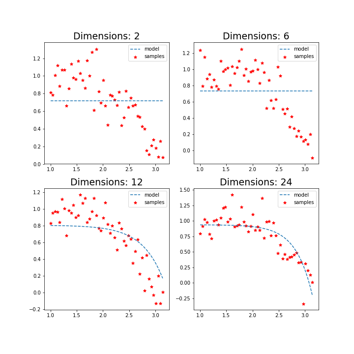
Lasso 回归
目标函数:
优化:为惩罚OLS每个w逐渐增加导致过度拟合的问题,新增的项为L1惩罚项(L1 Penalty)。
特点:比L2惩罚项严厉很多,可以产生稀疏回归参数,即多数回归参数为零。
1 | import matplotlib.pyplot as plt |
参考: