决策树

基本介绍

• 分而治之(divide-andconquer)：
  • 自根至叶的递归过程
  • 在每个中间结点寻找一个”划分”属性

• 过程：
  • 把数据集分成两组
  • 不同数据点被完美区分（Pure）开了么？
  • 不是：重复楼上两步
  • 是的：打完收⼯

建树逻辑

所有子树信息价值（信息熵、基尼指数等）的和必定小于等于原来整体数据集的信息价值，信息增益用来衡量减少的程度

def build(D=数据集)：

　　if D所有数据目标值 y 都相同：

　　　　return #递回停止条件

　　for i in D中的所有特征：

　　　　计算用i划分子树后获得的信息增益

　　if 所有特征都没有大于零的信息增益：

　　　　return #递回停止条件

　　被选择的特征 x = 具有最大信息增益的特征

　　for sub in 按照x划分子树后的数据集：

　　　　build(sub)

停止条件

• 当前结点包含的样本全属于同一类别，无须划分
• 当前属性集为空，或是所有样本在所有属性上取值相同，无法划分
• 当前结点包含的样本集合为空，不能划分

特性

• 优势：
  • ⾮⿊盒
  • 轻松去除⽆关attribute (Gain = 0)
  • Test起来很快 (O(depth))

• 劣势：
  • 只能线性分割数据
  • 贪婪算法 (每次分裂都选最好，有可能不是全局最好)

信息价值指标

信息熵

信息熵是度量样本集合”纯度”最常用的一种指标，假定当前样本集合D中第i类样本所占的比例为$P_i$，则D的信息熵定义为：

$$Ent(D)=-\sum_{i=1}^{n}{P_i \cdot log{P_i}}$$

• 某随机事件结果的种类越多，则该事件的熵越大（不确定性越大）
• 某随机事件的各种可能发生结果概率越均匀，则该事件的熵越大（不确定性越大）
• 值域：>= 0
• 缺点是计算量大（log）

信息增益(ID3)

$$Gain(D,a)=Ent(D)-\sum_{i=1}^{n}{\frac{|D^i|}{|D|}{Ent(D^i)}}$$

• 划分前的信息熵-划分后的总信息熵
• 越大越好

信息增益率(C4.5)

$$GainRatio(D,a)=\frac{Gain(D,a)}{IV(a)}$$ $$IV(a)=-\sum_{i=1}^{i}{\frac{|D^i|}{|D|}{log_2{\frac{|D^i|}{|D|}}}}$$

基尼指数(CART)

$$G=1-\sum_{i=1}^{n}{P_i^2}$$

• 值域：0~1

常见算法

• ID3：
  • 只能使用熵的信息增益处理离散特征的分类问题
  • 取值高的属性，更容易使数据更纯，其信息增益更大
  • 训练得到的是一棵庞大且深度浅的树（可以把N个数据分成100%纯洁的N组）

• C4.5：
  • 支持连续特征，在计算信息增益比之前首先将其离散化（与ID3差别）
  • 使用信息增益比的概念去除先选择多值特征的倾向
  • 在训练后检测训练集的正确分类比，并剪枝产生错误较多的叶子结点

• CART算法：
  • 使用基尼系数代替熵进行信息增益计算、只使用二叉树，并提供解决回归问题的能力
  • 以最小化不纯度，而不是最大化信息增益

DecisionTreeClassifier

from sklearn.tree import DecisionTreeClassifier
from sklearn import datasets
from sklearn.model_selection import train_test_split

iris = datasets.load_iris()
iris_data = iris['data']
iris_label = iris['target']
iris_target_name = iris['target_names']
X = np.array(iris_data)
Y = np.array(iris_label)

x_train, x_test, y_train, y_test = train_test_split(X, Y, test_size=0.25)

clf = DecisionTreeClassifier()
clf = clf.fit(x_train, y_train)

from sklearn.metrics import roc_curve, auc

y_pred = clf.predict(x_test)

false_positive_rate, true_positive_rate, thresholds = roc_curve(
    y_test, y_pred, pos_label=2)

roc_auc = auc(false_positive_rate, true_positive_rate)
roc_auc

1.0

调参

超参数：

• criterion: gini, entropy
• max_depth
• min_samples_split
• min_samples_leaf
• max_features
• max_leaf_nodes
• min_impurity_decrease

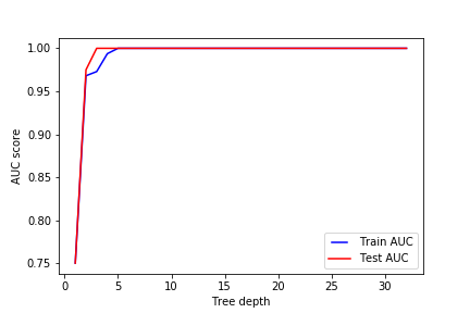
max_depth

要调整的第一个参数是max_depth（树的深度）。 树越深，它就分裂的越多，更能捕获有关数据的信息。 我们拟合一个深度范围从1到32的决策树，并绘制训练和测试auc分数

from matplotlib.legend_handler import HandlerLine2D
import matplotlib.pyplot as plt

max_depths = np.linspace(1, 32, 32, endpoint=True)
train_results = []
test_results = []

for max_depth in max_depths:
    dt = DecisionTreeClassifier(max_depth=max_depth)
    dt.fit(x_train, y_train)
    train_pred = dt.predict(x_train)
    false_positive_rate, true_positive_rate, thresholds = roc_curve(
        y_train, train_pred, pos_label=2)
    roc_auc = auc(false_positive_rate, true_positive_rate)

    train_results.append(roc_auc)
    y_pred = dt.predict(x_test)
    false_positive_rate, true_positive_rate, thresholds = roc_curve(
        y_test, y_pred, pos_label=2)
    roc_auc = auc(false_positive_rate, true_positive_rate)

    test_results.append(roc_auc)

line1, = plt.plot(max_depths, train_results, 'b', label='Train AUC')
line2, = plt.plot(max_depths, test_results, 'r', label='Test AUC')
plt.legend(handler_map={line1: HandlerLine2D(numpoints=2)})
plt.ylabel('AUC score')
plt.xlabel('Tree depth')

plt.savefig("../img/2019-07-29_决策树_1.png")
plt.close()

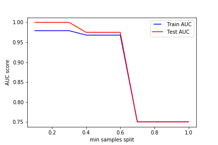
min_samples_split

min_samples_split表示拆分内部节点所需的最小样本数。 这可以在考虑每个节点处的至少一个样本，并考虑每个节点处的所有样本之间变化。 当我们增加此参数时，给与树更多的约束，因为它必须在每个节点处考虑更多样本。 在这里，我们将从10％到100％的样本中改变参数

min_samples_splits = np.linspace(0.1, 1.0, 10, endpoint=True)
train_results = []
test_results = []
for min_samples_split in min_samples_splits:
    dt = DecisionTreeClassifier(min_samples_split=min_samples_split)
    dt.fit(x_train, y_train)
    train_pred = dt.predict(x_train)
    false_positive_rate, true_positive_rate, thresholds = roc_curve(
        y_train, train_pred, pos_label=2)
    roc_auc = auc(false_positive_rate, true_positive_rate)
    train_results.append(roc_auc)
    y_pred = dt.predict(x_test)
    false_positive_rate, true_positive_rate, thresholds = roc_curve(
        y_test, y_pred, pos_label=2)
    roc_auc = auc(false_positive_rate, true_positive_rate)
    test_results.append(roc_auc)
from matplotlib.legend_handler import HandlerLine2D
line1, = plt.plot(min_samples_splits, train_results, 'b', label='Train AUC')
line2, = plt.plot(min_samples_splits, test_results, 'r', label='Test AUC')
plt.legend(handler_map={line1: HandlerLine2D(numpoints=2)})
plt.ylabel('AUC score')
plt.xlabel('min samples split')

plt.savefig("../img/2019-07-29_决策树_2.png")
plt.close()

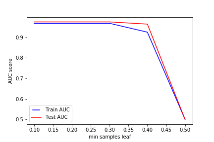
min_samples_leaf

min_samples_leaf是叶节点所需的最小样本数。 此参数类似于min_samples_splits，但是，这描述了叶子（树的基础）处的样本的最小样本数

min_samples_leafs = np.linspace(0.1, 0.5, 5, endpoint=True)
train_results = []
test_results = []
for min_samples_leaf in min_samples_leafs:
    dt = DecisionTreeClassifier(min_samples_leaf=min_samples_leaf)
    dt.fit(x_train, y_train)
    train_pred = dt.predict(x_train)
    false_positive_rate, true_positive_rate, thresholds = roc_curve(
        y_train, train_pred, pos_label=2)
    roc_auc = auc(false_positive_rate, true_positive_rate)
    train_results.append(roc_auc)
    y_pred = dt.predict(x_test)
    false_positive_rate, true_positive_rate, thresholds = roc_curve(
        y_test, y_pred, pos_label=2)
    roc_auc = auc(false_positive_rate, true_positive_rate)
    test_results.append(roc_auc)
from matplotlib.legend_handler import HandlerLine2D
line1, = plt.plot(min_samples_leafs, train_results, 'b', label='Train AUC')
line2, = plt.plot(min_samples_leafs, test_results, 'r', label='Test AUC')
plt.legend(handler_map={line1: HandlerLine2D(numpoints=2)})
plt.ylabel('AUC score')
plt.xlabel('min samples leaf')

plt.savefig("../img/2019-07-29_决策树_3.png")
plt.close()

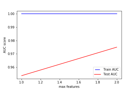
max_features

max_features表示查找最佳拆分时要考虑的要最大特征数量

max_features = list(range(1, len(iris_target_name)))
train_results = []
test_results = []
for max_feature in max_features:
    dt = DecisionTreeClassifier(max_features=max_feature)
    dt.fit(x_train, y_train)
    train_pred = dt.predict(x_train)
    false_positive_rate, true_positive_rate, thresholds = roc_curve(
        y_train, train_pred, pos_label=2)
    roc_auc = auc(false_positive_rate, true_positive_rate)
    train_results.append(roc_auc)
    y_pred = dt.predict(x_test)
    false_positive_rate, true_positive_rate, thresholds = roc_curve(
        y_test, y_pred, pos_label=2)
    roc_auc = auc(false_positive_rate, true_positive_rate)
    test_results.append(roc_auc)

from matplotlib.legend_handler import HandlerLine2D

line1, = plt.plot(max_features, train_results, 'b', label='Train AUC')
line2, = plt.plot(max_features, test_results, 'r', label='Test AUC')
plt.legend(handler_map={line1: HandlerLine2D(numpoints=2)})
plt.ylabel('AUC score')
plt.xlabel('max features')

plt.savefig("../img/2019-07-29_决策树_4.png")
plt.close()

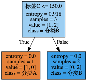
树的可视化

from IPython.display import display, Image
import graphviz
import pydotplus as pdp

dot_data = tree.export_graphviz(clf, out_file = None,
                               feature_names = ["标签A","标签B","标签C"],
                               class_names = ["分类A","分类B"],
                               filled = True,
                               rotate = False)

# 要先用brew install graphviz
graph = pdp.graph_from_dot_data(dot_data)
img = Image(graph.create_png())

参考：

1. 从机器学习到深度学习：基于Scikit-learn与TensorFlow的高效开发实战
2. 决策树（四）决策树调参